Tutorial for R Users

In this tutorial, we will go through CausalBGM workflow with the R package bayesgm.

First of all, you need to install , please refer to the install page to make sure bayesgm R package is installed.

Notes

bayesgm R package was developed based on reticulate package, which enables building R APIs based on Python APIs. Make sure the dependency R packages are installed.
The R APIs are consistent with Python APIs, detailed usage of CausalBGM APIs can be found at online document.

[1]:

library(bayesgm)

Dependencies

Reminder

Install the following dependent R packages for running the whole workflow.

[2]:

#install.packages(c("reticulate", "lattice", "Matrix", "R6","png"))

Notes

The function configure_bayesgm() specifies:

python: the path to the Python executable used by reticulate
pythonpath: the directory containing the bayesgm Python source code

Make sure to replace with your own paths here. After configuration, you can verify that the Python backend is available by running: stopifnot(bayesgm_available(configure = FALSE))

If the configuration is correct, this command will run silently; otherwise it will raise an error indicating that the Python environment or package cannot be located.

You may also run reticulate::py_config() to check which Python environment is currently being used by R.

[3]:

configure_bayesgm(
  python = "~/.conda/envs/py3.9/bin/python",
  pythonpath = "/home/ql339/project_pi_ql339/ql339/bayesgm/src"
)
stopifnot(bayesgm_available(configure = FALSE))

Binary treatment

We first give a step-by-step tutorial for implementing CausalBGM under binary treatment settings.

Data generation

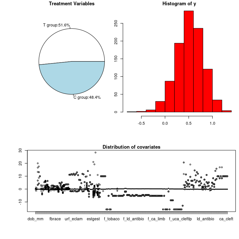
Let’s load a ACIC2018 simulation dataset (ufid=’629e3d2c63914e45b227cc913c09cebe’) with binary treatment.

The data contain treatment (X), potential outcome (Y), and covariates (V).

[4]:

data("acic_2018_example", package = "bayesgm")

ufid <- acic_2018_example$ufid
x <- acic_2018_example$x
y <- acic_2018_example$y
v <- acic_2018_example$v
ite_true <- acic_2018_example$ite_true
ate_true <- acic_2018_example$ate_true

Let’s take a look at the simulation data.

[5]:

par(cex=0.7, mai=c(0.1,0.1,0.2,0.1))
par(fig=c(0.1,0.5,0.5,1.0))
slices <- c(sum(x==1), sum(x==0))
lbls <- c(paste("T group:",round(sum(x==1)*100/length(x), 2), "%", sep=""), paste("C group:",round(sum(x==0)*100/length(x), 2), "%", sep=""))
pie(slices, labels = lbls, main="Treatment Variables")
par(fig=c(0.5,1,0.5,1), new=TRUE)
hist(y, breaks=12, col="red",xlab="y values")
par(fig=c(0.1,1.0,0.1,0.4), new=TRUE)
boxplot(v, main="Distribution of covariates", xlab="Covariate index", ylab="Values")

../_images/causalbgm_tutorial_r_12_0.png

Instantiate a CausalBGM model

Before creating a CausalBGM model, parameters are needed for configing a CausalBGM model, which are described as follows.

General Parameters

Config Parameter	Description
`dataset`	Dataset name to indicate the input data. Default: ‘Sim_Hirano_Imbens’.
`output_dir`	Output directory to save the results during the model training. Default: ‘.’.
`save_res`	Whether to save intermediate results. Default: TRUE.
`save_model`	Whether to save the model after training. Default: FALSE.
`binary_treatment`	Whether to use binary treatment settings. Default: FALSE.
`use_bnn`	Whether to use Bayesian neural networks. Default: TRUE.

Parameters for Iterative Updating Algorithm

Config Parameter	Description
`z_dims`	Latent dimensions of `Z`. Default: c(3L, 6L, 3L, 6L).
`v_dim`	Dimension of covariates. Default: 200.
`lr_theta`	Learning rate for updating model parameters. Default: 0.0001.
`lr_z`	Learning rate for updating latent variables. Default: 0.0001.
`g_units`	Number of units for covariates generative model. Default: c(64L, 64L, 64L, 64L, 64L).
`f_units`	Number of units for outcome generative model. Default: c(64L, 32L, 8L).
`h_units`	Number of units for treatment generative model. Default: c(64L, 32L, 8L).

Parameters for EGM Initialization

Config Parameter	Description
`kl_weight`	Coefficient for KL divergence term in BNNs. Default: 0.0001.
`lr`	Learning rate for EGM initialization. Default: 0.0002.
`g_d_freq`	Frequency for updating discriminators and generators. Default: 5.
`use_z_rec`	Whether to use reconstruction for latent features. Default: True.
`e_units`	Number of units for the encoder network. Default: c(64L, 64L, 64L, 64L, 64L).
`dz_units`	Number of units for the discriminator network in latent space. Default: c(64L, 32L, 8L).

[6]:

params <- list(
  dataset = "Semi_acic",
  output_dir = tempdir(),
  save_res = FALSE,
  save_model = FALSE,
  binary_treatment = TRUE,
  use_bnn = TRUE,
  z_dims = c(3L, 6L, 3L, 6L),
  v_dim = 177L,
  lr_theta = 0.0001,
  lr_z = 0.0001,
  g_units = c(64L, 64L, 64L, 64L, 64L),
  f_units = c(64L, 32L, 8L),
  h_units = c(64L, 32L, 8L),
  kl_weight = 0.0001,
  lr = 0.0002,
  g_d_freq = 5L,
  use_z_rec = TRUE,
  e_units = c(64L, 64L, 64L, 64L, 64L),
  dz_units = c(64L, 32L, 8L)
)

model <- CausalBGM(params = params, random_seed = NULL)

Model training

Train CausalBGM with an optional EGM warm-start.

Config Parameter	Description
`x`	Treatment, Required.
`y`	Outcome, Required.
`v`	Covariates, Required.
`batch_size`	Batch size for training. Default: 32.
`epochs`	Number of epochs for training. Default: 100.
`epochs_per_eval`	Frequency of evaluations during training (e.g., every 5 epochs). Default: 5.
`use_egm_init`	Whether to run EGM initialization before iterative training. Default: True.
`epochs_per_eval`	Frequency of evaluations during training (e.g., every 5 epochs). Default: 5.
`egm_n_iter`	Number of EGM initialization iterations. Default: 30000.
`egm_batches_per_eval`	Evaluate EGM initialization every this many iterations. Default: 500.
`verbose`	Controls verbosity level, showing progress and evaluation metrics. Default: 1.

Notes

The training procedure consists of two phases:

EGM initialization (optional) — warm-start to obtain a good starting point for the latent variables and model parameters. This phase is optional and can be skipped by setting use_egm_init to False.
Stochastic iterative updating — alternates between updating the generator network parameters and the per-sample latent variables via stochastic gradient optimization.

[7]:

model <- model$fit(
    x = x,
    y = y,
    v = v,
    epochs = 100L,
    epochs_per_eval = 10L,
    batch_size = 32L,
    use_egm_init = TRUE,
    egm_n_iter = 30000L,
    egm_batches_per_eval = 500L,
    verbose = 1L
)

Model Prediction

Estimate causal effects with posterior intervals from latent MCMC samples.

Config Parameter	Description
`x`	Treatment, Required.
`y`	Outcome, Required.
`v`	Covariates, Required.
`alpha`	Significance level for the posterior interval. Default: 0.01.
`n_mcmc`	Number of posterior MCMC samples to draw. Default: 3000.
`burn_in`	Number of burn-in MCMC samples before drawing. Default: 5000.
`q_sd`	Standard deviation for the proposal distribution used in Metropolis-Hastings (MH) sampling. Default: 1.0.
`sample_y`	Whether to consider the variance function in the outcome generative model. Default: True.
`bs`	Batch size in inference stage, denoting number of test subjects processed per batch prediction. Default: 10000.

Return	Type	Description	Shape
`res$effect`	`numeric vector`	Point estimates of the Individual Treatment Effect (ITE).	`(length(x))`
`res$interval`	`numeric matrix`	Posterior intervals for the ITEs, representing `[lower bound, upper bound]`	`(length(x), 2)`

[8]:

res <- model$predict(
    x = x,
    y = y,
    v = v,
    alpha = 0.01,
    n_mcmc = 3000L,
    burn_in = 5000L,
    q_sd = 1.0
)
pred_ite <- as.numeric(res$effect)
pred_interval <- as.matrix(res$interval)

Model Evaluation

For this ACIC example, the package dataset includes the ground-truth counterfactual outcomes, so the true individual treatment effects and average treatment effect are available directly.

[9]:

pred_ate <- mean(pred_ite)
delta_ate <- abs(pred_ate - ate_true)
delta_pehe <- mean((pred_ite - ite_true)^2)


cat(sprintf(
  "Delta ATE (Absolute Error in Average Treatment Effect): %.4f\n",
  delta_ate
))
cat(sprintf(
  "Delta PEHE (Precision in Estimation of Heterogeneous Effect): %.4f\n",
  delta_pehe
))

Delta ATE (Absolute Error in Average Treatment Effect): 0.0037
Delta PEHE (Precision in Estimation of Heterogeneous Effect): 0.0002

Continuous treatment

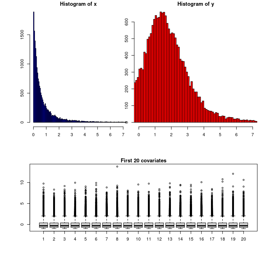
We first give a step-by-step tutorial for implementing CausalBGM under continuous treatment settings. We use the Hirano and Imbens simulation dataset for an example.

[10]:

sim_data <- load_sim_hirano_imbens(N = 20000L, v_dim = 200L, seed = 0L)

x <- sim_data$x
y <- sim_data$y
v <- sim_data$v
grid_val <- seq(0, 3, length.out = 20)
true_effect <- grid_val + 2 * (1 + grid_val)^(-3)

Let’s take a look at the simulation data.

[11]:

par(cex=0.7, mai=c(0.1,0.1,0.2,0.1))
par(fig=c(0.1,0.5,0.5,1.0))
hist(x, breaks="FD", xlim=c(0,7), col="blue",xlab="x values")
par(fig=c(0.5,1,0.5,1), new=TRUE)
hist(y, breaks="FD", xlim=c(0,7), col="red",xlab="y values")
par(fig=c(0.1,1.0,0.1,0.4), new=TRUE)
boxplot(v[,1:20],main="First 20 covariates", xlab="Covariate index", ylab="v values")

../_images/causalbgm_tutorial_r_25_0.png

Instantiate a CausalBGM model

[12]:

params <- list(
  dataset = "Sim_Hirano_Imbens",
  output_dir = tempdir(),
  save_res = FALSE,
  save_model = FALSE,
  binary_treatment = FALSE,
  use_bnn = TRUE,
  z_dims = c(1L, 1L, 1L, 7L),
  v_dim = 20L,
  lr_theta = 0.0001,
  lr_z = 0.0001,
  g_units = c(64L, 64L, 64L, 64L, 64L),
  f_units = c(64L, 32L, 8L),
  h_units = c(64L, 32L, 8L),
  kl_weight = 0.0001,
  lr = 0.0002,
  g_d_freq = 5L,
  use_z_rec = TRUE,
  e_units = c(64L, 64L, 64L, 64L, 64L),
  dz_units = c(64L, 32L, 8L)
)

model <- CausalBGM(params = params, random_seed = NULL)

Model Training

Train CausalBGM with an optional EGM warm-start.

Config Parameter	Description
`x`	Treatment, Required.
`y`	Outcome, Required.
`v`	Covariates, Required.
`batch_size`	Batch size for training. Default: 32.
`epochs`	Number of epochs for training. Default: 100.
`epochs_per_eval`	Frequency of evaluations during training (e.g., every 5 epochs). Default: 5.
`use_egm_init`	Whether to run EGM initialization before iterative training. Default: True.
`epochs_per_eval`	Frequency of evaluations during training (e.g., every 5 epochs). Default: 5.
`egm_n_iter`	Number of EGM initialization iterations. Default: 30000.
`egm_batches_per_eval`	Evaluate EGM initialization every this many iterations. Default: 500.
`verbose`	Controls verbosity level, showing progress and evaluation metrics. Default: 1.

[13]:

model <- model$fit(
    x = x,
    y = y,
    v = v,
    epochs = 100L,
    epochs_per_eval = 10L,
    batch_size = 32L,
    use_egm_init = TRUE,
    egm_n_iter = 30000L,
    egm_batches_per_eval = 500L,
    verbose = 1L
)

Model Prediction

Estimate causal effects with posterior intervals from latent MCMC samples.

Config Parameter	Description
`x`	Treatment, Required.
`y`	Outcome, Required.
`v`	Covariates, Required.
`alpha`	Significance level for the posterior interval. Default: 0.01.
`n_mcmc`	Number of posterior MCMC samples to draw. Default: 3000.
`burn_in`	Number of burn-in MCMC samples before drawing. Default: 5000.
`x_values`	Treatment value(s) for dose-response function to be predicted. Examples: 1.0 or c(1.0, 2.0)
`q_sd`	Standard deviation for the proposal distribution used in Metropolis-Hastings (MH) sampling. Default: 1.0.
`sample_y`	Whether to consider the variance function in the outcome generative model. Default: True.
`bs`	Batch size in inference stage, denoting number of test subjects processed per batch prediction. Default: 10000.

Return	Type	Description	Shape
`res$effect`	`numeric vector`	Point estimates of the Average Dose-Response Function.	`(length(x_values))`
`res$interval`	`numeric matrix`	Posterior intervals for the ADRF, representing `[lower bound, upper bound]`	`(length(x_values), 2)`

[14]:

res <- model$predict(
    x = x,
    y = y,
    v = v,
    alpha = 0.05,
    x_values = grid_val,
    n_mcmc = 3000L,
    burn_in = 5000L,
    q_sd = 1.0
)

pred_effect <- as.numeric(res$effect)
pred_interval <- as.matrix(res$interval)
pred_lower <- pred_interval[, 1]
pred_upper <- pred_interval[, 2]

Model Evaluation

[15]:

rmse <- sqrt(mean((true_effect - pred_effect)^2))
mape <- mean(abs((true_effect - pred_effect) / true_effect))

cat(sprintf(
  "RMSE (Root Mean Squared Error): %.4f\n",
  rmse
))
cat(sprintf(
  "MAPE (Mean Absolute Percentage Error): %.4f\n",
  mape
))

RMSE (Root Mean Squared Error): 0.0289
MAPE (Mean Absolute Percentage Error): 0.0110

Plot of the average dose-response function (ADRF)

We now compare plot of the true ADRF and the ADRF estimated by our model.

[16]:

plot(
  grid_val,
  true_effect,
  type = "n",
  ylim = range(c(true_effect, pred_lower, pred_upper), finite = TRUE),
  xlab = "Treatment level",
  ylab = "ADRF",
  main = "Predicted and True ADRF"
)
polygon(
  x = c(grid_val, rev(grid_val)),
  y = c(pred_lower, rev(pred_upper)),
  border = NA,
  col = grDevices::adjustcolor("firebrick", alpha.f = 0.2)
)
lines(grid_val, true_effect, col = "black", lwd = 2)
lines(grid_val, pred_effect, col = "firebrick", lwd = 2)
legend(
  "bottomright",
  legend = c("True ADRF", "Predicted ADRF", "Predicted 95% interval"),
  col = c("black", "firebrick", NA),
  lty = c(1, 1, NA),
  lwd = c(2, 2, NA),
  pch = c(NA, NA, 15),
  pt.cex = c(NA, NA, 2),
  pt.bg = c(NA, NA, grDevices::adjustcolor("firebrick", alpha.f = 0.2)),
  bty = "n"
)

../_images/causalbgm_tutorial_r_35_0.png

[17]:

sessionInfo()

R version 4.4.2 (2024-10-31)
Platform: x86_64-pc-linux-gnu
Running under: Red Hat Enterprise Linux 8.10 (Ootpa)

Matrix products: default
BLAS/LAPACK: FlexiBLAS OPENBLAS;  LAPACK version 3.12.0

locale:
 [1] LC_CTYPE=en_US.UTF-8       LC_NUMERIC=C
 [3] LC_TIME=en_US.UTF-8        LC_COLLATE=en_US.UTF-8
 [5] LC_MONETARY=en_US.UTF-8    LC_MESSAGES=en_US.UTF-8
 [7] LC_PAPER=en_US.UTF-8       LC_NAME=C
 [9] LC_ADDRESS=C               LC_TELEPHONE=C
[11] LC_MEASUREMENT=en_US.UTF-8 LC_IDENTIFICATION=C

time zone: America/New_York
tzcode source: system (glibc)

attached base packages:
[1] stats     graphics  grDevices utils     datasets  methods   base

other attached packages:
[1] bayesgm_0.1.0

loaded via a namespace (and not attached):
 [1] crayon_1.5.3      vctrs_0.6.5       cli_3.6.3         rlang_1.1.4
 [5] png_0.1-8         jsonlite_1.8.9    glue_1.8.0        htmltools_0.5.8.1
 [9] IRdisplay_1.1     IRkernel_1.3.2    fansi_1.0.6       grid_4.4.2
[13] evaluate_1.0.1    fastmap_1.2.0     base64enc_0.1-3   lifecycle_1.0.4
[17] compiler_4.4.2    Rcpp_1.0.13-1     pbdZMQ_0.3-14     lattice_0.22-9
[21] digest_0.6.37     R6_2.6.1          repr_1.1.7        reticulate_1.45.0
[25] utf8_1.2.4        pillar_1.9.0      Matrix_1.7-4      uuid_1.2-2
[29] tools_4.4.2       withr_3.0.2